Analysis Tools¶

The Analysis tools tab enriches the loaded dataset by running computations as asynchronous background jobs. Each job either adds new columns to the dataset or replaces existing XYZ geometries with optimized versions.

Note

A compiled dataset must be present (loaded via the Data Manager) before running any tool.

Analysis tools workspace

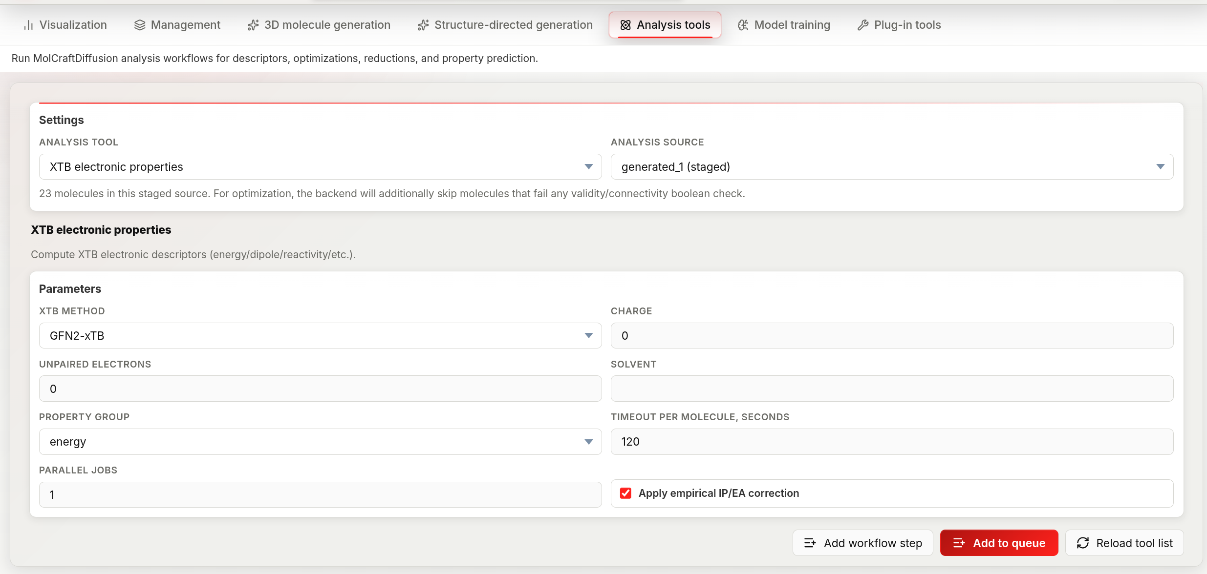
The Analysis tools workspace: pick a tool and source under Settings, configure its parameters, then queue and run the step.

General workflow¶

The tab is organized around a step queue:

1 Settings — pick the Analysis tool and the Analysis source (which dataset/staged source to run on).
2 Parameters — configure the tool's parameters, then click Add to queue. Repeat to chain several steps (e.g. XYZ to SMILES → validity → xTB).
Each queued step has a Post action: No post-action, Apply results (merge new columns into the dataset when the step completes), or Register optimized set (add the result as a staged source in the Data Manager — used for geometry optimization outputs).
In the Workflow panel, click Run. Steps execute one at a time as background jobs; you can navigate to other tabs while waiting. Pause, Cancel active, and Clear workflow control the run; a paused or failed workflow shows Resume instead of Run.
Completed jobs appear in the Analysis queue panel with a status badge (queued / running / completed / failed / cancelled) and a log/terminal button to inspect the raw output. If a step ran without a post action, you can still click Apply results (or Apply all results) or Register optimized set there afterwards.

Cancelling: click Cancel on a queued or running job. Clear queue removes finished jobs from the list.

Recommended run order¶

Many tools depend on outputs from earlier ones:

XYZ to SMILES — produces the smiles column required by validity checks and similarity filters.
Validity and connectivity metrics — use SMILES + XYZ to flag bad geometries; filter these out before expensive calculations.
XTB geometry optimization (optional) — replace raw geometries with optimized ones before running single-point calculations.
XTB electronic properties — single-point calculations on the (optionally optimized) geometries.
Featurize — compute SOAP or UMA vectors.
Dimensionality reduction — project featurization vectors to 2D for visualization.
Predict properties — run a MolCraftDiffusion checkpoint for property inference.

Tool reference¶

Validity and connectivity metrics¶

Checks each molecule's geometry and connectivity against a set of chemical rules and flags problems as boolean columns.

Metric sets define which rules are applied:

Metric set	What it checks
`core`	Basic valence rules, bond lengths, formal charges
`posebuster`	Core checks + pose-level geometry (torsions, clashes, planarity)
`geom_revised`	Revised geometry thresholds from the geom_revised benchmark

Parameter	Default	Options	What it does
Metric set	`posebuster`	core, posebuster, geom_revised	Rule set to apply
Recheck topology with RDKit	false	boolean	Re-evaluate bond connectivity using RDKit after the initial parse. Useful if `xyz2mol` assigns bonds incorrectly
Molecule converter	`xyz2mol`	xyz2mol, openbabel	Algorithm used to infer bonds from XYZ coordinates. Switch to `openbabel` if `xyz2mol` fails for your element types

Output: one boolean column per validity criterion (True = passes the check). Failed molecules are False.

XYZ to SMILES conversion¶

Converts each molecule's XYZ geometry to a SMILES string (Simplified Molecular Input Line Entry System — a compact linear notation for molecular connectivity, e.g. CCO = ethanol). Also computes two derived representations:

Morgan fingerprint — a fixed-length binary vector encoding each atom's local chemical environment up to a given bond radius. Used as a numerical molecular representation for similarity search and machine learning.

Bemis–Murcko scaffold — the core ring-and-linker framework of a molecule stripped of all side chains. Used to group molecules by structural class.

Parameter	Default	Range	What it does
Morgan fingerprint bits	2048	integer	Length of the fingerprint vector. 1024–4096 are typical values; longer vectors are more discriminating but use more memory

Output columns added: smiles, morgan_fp (vector), scaffold (SMILES string of the ring system).

Run this tool first — the smiles column enables SMARTS and similarity filters in the Visualization tab.

XTB electronic properties¶

Runs xTB (extended tight-binding) single-point quantum-chemical calculations. xTB is a fast semi-empirical method that gives approximate but chemically meaningful electronic descriptors in seconds per molecule.

xTB methods available:

Method	Speed	Accuracy	Best for
GFN1-xTB	Fastest	Lower	Large datasets, initial screening
GFN2-xTB	Moderate	Higher	General-purpose; recommended default
PTB	Fastest	Moderate	Very large systems where GFN2 is too slow

Parameter	Default	Options	What it does
XTB method	GFN2-xTB	GFN1-xTB, GFN2-xTB, PTB	Level of theory
Charge	0	integer	Net formal charge of all molecules in the dataset. If molecules have different charges, pre-split the dataset
Unpaired electrons	0	integer	Number of unpaired electrons (0 = closed-shell, the typical case for drug-like molecules)
Solvent	(empty)	string	Implicit solvent name (e.g. `water`, `acetonitrile`, `methanol`). Leave empty for gas-phase calculation
Property group	`energy`	see below	Which property set to compute
Timeout per molecule	120 s	integer	Maximum wall time before marking a molecule as failed. Increase for large or complex structures
Parallel jobs	1	integer	Number of molecules calculated simultaneously. Set to the number of CPU cores available
Apply empirical correction	true	boolean	Apply Grimme's empirical correction to ionisation potential and electron affinity values

Property groups:

Group	Columns added
`energy`	Total energy (Hartree), HOMO energy, LUMO energy, HOMO–LUMO gap
`dipole`	Dipole moment magnitude (Debye)
`reactivity`	Ionisation potential (IP), electron affinity (EA), chemical potential (μ), hardness (η), softness (S), electrophilicity (ω)
`global`	Combined energy + reactivity descriptors
`charges`	Per-atom partial charges (added as a vector column)
`fukui`	Fukui electrophilic (f⁻) and nucleophilic (f⁺) indices (per-atom vector columns)
`bond_orders`	Mayer bond orders for all atom pairs (vector column)
`all`	All of the above

Start with energy for a quick screen; add reactivity if you need IP/EA/hardness; use all for a comprehensive descriptor set before featurization.

XTB geometry optimization¶

Relaxes each molecule's geometry to a local energy minimum. The output either replaces the original XYZ coordinates in-place or is registered as a new staged source.

MMFF94 (Merck Molecular Force Field 94): a classical force field optimized for drug-like organic molecules. Faster than xTB but less accurate for heteroatoms, strained systems, or unusual bonding.

Parameter	Default	Options	What it does
Optimization level	`gfn2`	gfn1, gfn2, gfn-ff, mmff94	Method for geometry relaxation. GFN2 is the recommended default; use mmff94 for very large molecules or if xTB is too slow
Charge	0	integer	Net formal charge
Timeout per molecule	240 s	integer	Maximum wall time. Optimization is slower than single-point; increase for large structures
Covalent radii scale factor	1.3	float	Scale applied to covalent radii when assigning bonds from XYZ coordinates. Increase (e.g. to 1.5) if bonds between distant atoms are being missed

After the job completes, choose: - Apply results — overwrites the current XYZ geometries for those molecule IDs in-place. - Register optimized set — adds the optimized geometries as a staged source in the Data Manager. Behavior depends on the ID prefix and Data source label fields:

ID prefix	Data source label	Result
Empty	Same as the original data source	Replacement mode — original source rows are removed; optimized rows take their place
Non-empty	Different from the original data source	Append mode — optimized rows are added as a new staged source with the prefix prepended to their IDs; the label must not already exist

Featurize¶

Computes a fixed-length numeric vector for each molecule, used as input for dimensionality reduction or external ML models.

SOAP (Smooth Overlap of Atomic Positions): encodes each atom's local chemical environment as a rotationally invariant power spectrum, then pools per-atom descriptors into one vector per molecule. Purely geometry-based — no SMILES needed.

UMA: a neural network–based featurizer that produces dense molecular embeddings.

Morgan fingerprint: computes a Morgan (circular) fingerprint directly from a SMILES column via RDKit — runs in-process, no XYZ or GPU required. Needs an existing SMILES column (e.g. from XYZ to SMILES conversion).

Parameter	Default	Applies to	What it does
Backend	`soap`	all	Choose SOAP (geometry-based), UMA (neural), or Morgan fingerprint (SMILES-based)
Auto-detect species	true	SOAP	Automatically infer the element list from the dataset. Disable to specify elements manually for reproducible vectors across datasets with different compositions
r_cut	6.0 Å	SOAP	Cutoff radius for the local atomic environment. Larger values capture longer-range interactions but increase vector length
n_max	8	SOAP	Number of radial basis functions. Higher = finer radial resolution
l_max	6	SOAP	Maximum angular momentum (spherical harmonic order). Higher = finer angular resolution. Computational cost scales as (l_max + 1)²
sigma	0.1	SOAP	Gaussian smearing width for atomic densities. Larger sigma smooths out geometry noise
Pooling	`mean`	SOAP, UMA	How per-atom descriptors are combined into one vector: `mean` (average) or `sum` (total)
UMA model path	(empty)	UMA	Optional path to a local UMA checkpoint. Relative paths resolve from the repository root; leave empty for the default checkpoint
UMA device	`cpu`	UMA	`auto` selects GPU if available; `cpu` forces CPU; `cuda` forces GPU
UMA batch size	8	UMA	Number of molecules processed per GPU batch
SMILES column	(required)	Fingerprint	Dataset column holding SMILES strings to fingerprint
Morgan radius	2	Fingerprint	Circular fingerprint radius (bond hops considered around each atom)
Morgan bits	2048	Fingerprint	Length of the fingerprint vector
Use chirality	false	Fingerprint	Encode stereochemistry in the fingerprint
Use feature invariants	false	Fingerprint	Use pharmacophoric feature invariants instead of plain atom types

Output: a vector column added to the dataset. This column is the required input for Dimensionality reduction.

Dimensionality reduction¶

Projects a high-dimensional molecular vector column to two numeric coordinates (e.g. dim_red_x, dim_red_y) that can be used as scatter plot axes in the Visualization tab.

UMAP (Uniform Manifold Approximation and Projection): preserves both local neighbourhood structure and global topology. Faster than t-SNE for large datasets. Distances in the 2D plot are more interpretable.

t-SNE (t-distributed Stochastic Neighbor Embedding): prioritises local cluster structure. Better at revealing tight clusters, but global distances are not meaningful and results vary with random seed.

Parameter	Default	Applies to	What it does
Vector column	(required)	both	The featurization column to project
Algorithm	UMAP	both	UMAP or t-SNE
Metric	`euclidean`	both	Distance metric: `euclidean`, `cosine`, or `manhattan`. Use `cosine` for high-dimensional sparse vectors (e.g. Morgan fingerprints)
Random seed	42	both	Fix for reproducibility

UMAP-specific:

Parameter	Default	What it does
Neighbors	15	Number of nearest neighbours in the high-dimensional space. Smaller = finer local structure; larger = more global view
Min distance	0.1	Minimum distance between points in 2D. Smaller = tighter clusters
Epochs	0 (auto)	Optimisation iterations; 0 lets UMAP choose based on dataset size
Learning rate	1.0	Step size for the embedding optimiser
Spread	1.0	Overall scale of the 2D embedding
Low memory	true	Use a slower but memory-efficient graph construction algorithm; keep enabled for datasets > 10 000 molecules

t-SNE-specific:

Parameter	Default	What it does
Device	CPU	`CPU (openTSNE)` or `CUDA (tsne-cuda)` — GPU can be 10–100× faster for large datasets
CUDA device	0	GPU index when device = CUDA
Perplexity	30	Effective number of neighbours; typical range 5–50. Increase for large, dense datasets
Learning rate	200	Gradient step size. If the embedding collapses to a ball, increase this value
Iterations	1 000	Total optimisation steps. Increase for large datasets
Early exaggeration	12.0	Amplification of inter-cluster distances in the early optimisation phase — helps clusters separate
Theta	0.5	Barnes–Hut approximation (0 = exact but slow; 1 = fastest but less accurate)
Initialization	PCA	Starting layout for the embedding: `PCA` (recommended, deterministic), `Random`, or `Spectral`
Parallel jobs	1	CPU threads for openTSNE

Output: two numeric columns added to the dataset, e.g. dim_red_x and dim_red_y. Bind these to the X/Y axes of a scatter plot in the Visualization tab to see the chemical space layout.

Predict properties¶

Runs property inference using a MolCraftDiffusion checkpoint. Only models that expose property predictors (CFG-trained models) appear in the list.

Parameter	Options	What it does
Predictive model	select from available checkpoints	The checkpoint used for inference

Output: one numeric column per predicted property, added to the dataset.

This is useful for predicting properties on a new set of molecules (e.g. generated structures) using a model trained on labelled data.